[New post] Data Science: Deep Learning with Tensor Flow
ants123456789 posted: " As we learn the python for financial world, we will want to go into what is the future domain that is being explored to bring prediction of the securities much like human. Able to react and re-learn, scientists are working on deep learning base on neuron"
As we learn the python for financial world, we will want to go into what is the future domain that is being explored to bring prediction of the securities much like human. Able to react and re-learn, scientists are working on deep learning base on neurons of brain. Having a large of neurons like a neutral network to sensor every signal.
Short Introduction on Neural Network
A neural network is a network or circuit of neurons.
An artificial neural network, composed of artificial neurons or nodes.
Thus a neural network is either a biological neural network, made up of biological neurons, or an artificial neural network, for solving artificial intelligence (AI) problems.
Frank Rosenblatt, an American psychologist, conceptualized and tried to build a machine that responds like the human mind in 1958. He named his machine "Perceptron."
An artificial neural network in its basic form has three layers of neurons.
Information flows from one to the next, just as it does in the human brain:
The input layer: the data's entry point into the system
The hidden layer: where the information gets processed
The output layer: where the system decides how to proceed based on the data
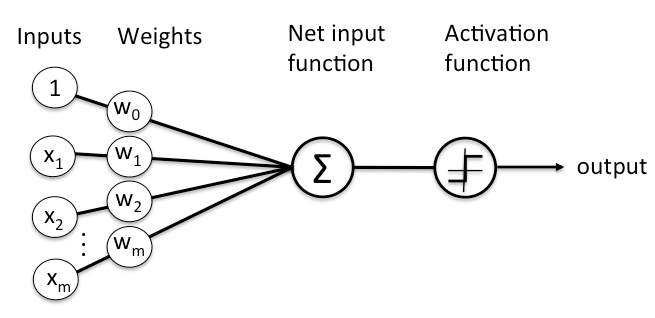
In an artificial neural network, the artificial neuron receives a stimulus in the form of a signal that is a real number. Then, output of each neuron is computed by a nonlinear function of the sum of its inputs.
Adds up the value of every neurons from the previous column it is connected to.
There are Xn inputs (x1, x2, x3) coming to the neuron.
This value is multiplied, by another variable called "weight" (w1, w2, w3) which determines the connection between the two neurons.
A bias value may be added to the total value calculated.
After all those summations, the neuron finally applies a function called "activation function" to the obtained value.
This activation function comes with non-linear properties. 3 common activation functions:
Sigmoid activation
Tanh action
Rectified linear unit (ReLu)
How does a neural network learn ?
The most basic neural network is called perception.
It consists on 2 neurons in the inputs column and 1 neuron in the output column.
Training multiple layers perception networks is much more complicated. With the simple perceptron, we could easily evaluate how to change the weights according to the error.
The solution to optimizing weights of a multi-layered network is known as backpropagation.
The output of the network is generated in the same manner as a perceptron.
The inputs multiplied by the weights are summed and fed forward through the network.
The difference here is that they pass through additional layers of neurons before reaching the output
Using TensorFlow
TensorFlow is a free and open-source software library for machine learning and artificial intelligence.
It can be used across a range of tasks but has a particular focus on training and inference of deep neural networks.
There is an online Tensorflow playground for you to try so you need not install tensorflow on you PC computer.
Let work a example on using tensorflow.
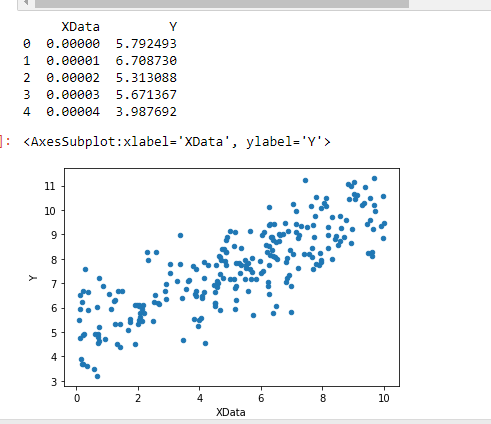
After warm up on above example of tensorflow. We continue to work on linear regression using tensorflow.
Finally, you are now learn how deep learning using tensorflow V2 for linear regression. There is important things to take note, on Tensorflow V2. The programming function may have issue when you using V2 when you will need to access V1 function. One of the way is using tf.compat.v1., if not, you may have to rewrite to V2 format.


No comments:
Post a Comment
Note: Only a member of this blog may post a comment.